Dice Algebra

by Caio Mizerkowski

14 min read

Criei a Álgebra de Dados como um toolkit para me ajudar a modelar o comportamento das distribuições de dados em jogos de RPG, assim como para modelar as operações realizadas entre estas distribuições. A maior parte do que está presente nesse documento é só a formalização de operações já conhecidas e usadas nos mais diversos jogos de RPG, somente com uma notação um pouco mais formal e “matematizada”. A utilidade disso para mim é facilitar o desenvolvimento de um programa para gerar a distribuição de probabilidade da combinação de dados e a suprir as minhas necessidades emocionais de encapsular o que eu já conhecia de forma mais completa. Peço já desculpas por qualquer uso inadequado da linguagem matemática.

Podemos dizer que esse documento descreve as operações de adição, deslocamento, multiplicação e mistura de distribuições de modo a facilitar a implementação das mesmas em um programa de computador.

Sumário:

• 1. The Underlying Set
  • 1.1 Delta‑Distributions
• 2. Core Operations
  • 2.1 Convolution (Sum of Independent Rolls)
  • 2.2 \(n\)-Fold Convolution (Roll \(n\) Times)
  • 2.3 Scaling
  • 2.4 Shift
• 4. Embedding Integers into \(\\mathcal{D}\)
  • 4.1 The Embedding Map
  • 4.2 Recovering Integer Addition
  • 4.3 Recovering Integer Multiplication
  • 4.4 Shifts as Delta‑Convolution
  • 4.5 Why This Matters
  • 4.6 Note on integers vs. delta‑distributions
• 5. Algebraic Laws
  • 5.1 Identities
  • 5.2 Commutativity
  • 5.3 Associativity
  • 5.4 Distributivity
  • 5.5 Shift Semigroup
• 6. Worked Examples
  • 6.1 Basic Dice Tables
    • 6.1.1 One Six‑Sided Die (1d6)
    • 6.1.2 Sum of Two d6’s (2d6)
    • 6.1.3 Scaling a d6 by 2 (2*1d6)
• 7. Extended Operations
  • 7.1 Reflection / Negation
  • 7.2 Convolution with Reflection (｢Difference｣)
  • 7.3 Pointwise Sum
    • 7.3.1
    • 7.3.2
    • 7.3.3
  • 7.4 The Mixture Kernel \(M(k)\)
    • 7.4.1 Definition
    • 7.4.2 Example
• 8. Delta Distributions and Scalar Embedding
  • 8.1 Delta Distributions
  • 8.2 Numbers as Deltas
• 9. Summary and Structure of Dice Algebra
  • 9.1 Core Structures
  • 9.2 Extended Operations

1. The Underlying Set

O universo \(\mathcal{D}\) analisado é o conjunto de distribuições de probabilidade discretas e finitas sobre os números inteiros \(\mathbb{Z}\).

O valor \(k\in\mathbb{Z}\) é o resultado, com valores no intervalo \((-\infty,+\infty)\).

A distribuição \(X\) é uma função que associa a cada resultado \(k\) uma probabilidade \(X(k)\), com valores no intervalo \([0,1]\). Cada distribuição \(X\) tem suporte finito, ou seja, \(X(k)\) é diferente de zero para apenas um número finito de valores de \(k\) e a soma de todas as probabilidades é igual a 1:

\[\mathcal{D} = \Bigl\{ \,X:\mathbb{Z}\to[0,1]\; \Big| \;\sum_{k\in\mathbb{Z}}X(k)=1, \;X(k)=0\text{ for all but finitely many }k \Bigr\}.\]

Alguns exemplos de distribuições \(X\in\mathcal{D}\):

• \(X=1d6\): é a distribuição uniforme:

  \[1d6(k) = \begin{cases} \tfrac16, & k=1,2,3,4,5,6,\\ 0, & \text{otherwise.} \end{cases}\]

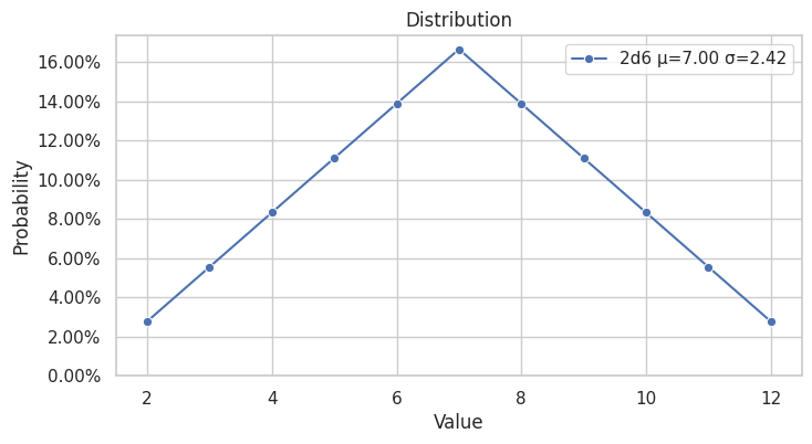
• \(X=2d6\): é a distribuição triangular formada pela adição entre duas distribuições uniformes.

1.1 Delta‑Distributions

Para lidar com os números inteiros \(\mathbb{Z}\) presentes em jogos de RPG, foi necessário mapear estes como deltas. Todo número inteiro \(n\) passa a ser representado por meio de uma distribuição \(\delta_n\in\mathcal{D}\), onde \(\delta_n\) é a distribuição delta que tem suporte apenas em \(n\):

\[\delta_n(k) = \begin{cases} 1, & k = n,\\ 0, & \text{otherwise.} \end{cases}\]

Casos especiais:

• \(\delta_0\) é a distribuição ｢zero｣, é a identidade para operações análogas à soma,
• \(\delta_1\) é a distribuição ｢unitária｣, é a identidade para operações análogas à multiplicação.

Exemplo para \(\delta_3\), somente o resultado \(3\) tem probabilidade diferente de zero:

\(k\)	\(\delta_3(k)\)
0	0
1	0
2	0
3	1
4	0

2. Core Operations

Foram definidas quatro maneiras fundamentais de se combinar as distribuições pertencentes a \(\mathcal{D}\). E por meio delas se procurou expressar as principais maneiras de se ｢somar｣ e ｢escalar｣ um conjunto de dados em um jogo de RPG. Elas podem parecer um tanto complexas ao serem expressas por meio de funções, mas quase todas elas são operações simples e intuitivas em um jogo de RPG.

2.1 Convolution (Sum of Independent Rolls)

A operação que resulta na soma de duas distribuições é chamada de Convolução. Essa operação representa o lançamento de dois dados independentes e a soma dos resultados. Um exemplo é lançar \(1d20+1d8\).

Notação:

\[Z = X + Y\]

Definição:

Para cada resultado \(k\), existe um conjunto de pares ordenados \((i,j)\) cuja soma é igual a \(k\). Portanto, caso o resultado \(i\) seja obtido em \(X\), é necessário que o resultado \(j=k-i\) seja obtido em \(Y\), e a probabilidade desse evento é \(X(i)Y(j)\). Essa lógica é válida para todos os pares \((i,j)\) cuja soma é \(k\), e a probabilidade de \(Z(k)\) é a soma de \(X(i)Y(j)\) para todos os pares \((i,j): i+j=k\). Portanto:

\[Z(k) \;=\; \sum_{i + j = k} X(i)\,Y(j).\]

A probabilidade \(Z(k)\) é a soma de todas as probabilidades \(X(i)Y(j)\) em que o resultado \(k\) é igual ao resultado \(i+j\).

Esse processo é equivalete a convolução discreta entre duas funções:

\[[f * g](k) = \sum_{i=-\infty}^{\infty} f[i] \cdot g[k - i]\]

Exemplo: Para \(Z = 1d4 + 1d6\), a probabilidade de \(Z(5)\) é dada por:

\[Z(5) =\sum_{i+j=5}1d4(i)\,1d6(j)\]

Aonde \((i,j)\in\{(1,4),(2,3),(3,2),(4,1)\}\). Portanto:

\[RHS: 1d4(1)\,1d6(4) + 1d4(2)\,1d6(3) + 1d4(3)\,1d6(2) + 1d4(4)\,1d6(1)\] \[Z(5) = 4\cdot\tfrac{1}{4}\cdot\tfrac{1}{6} =\tfrac{1}{6}\]

2.2 \(n\)-Fold Convolution (Roll \(n\) Times)

Assim como o produto pode ser visto como a repetição da soma, a operação de \(n\)-Fold Convolution é a repetição da operação de convolução \(n\) vezes para a distribuição \(X\). Essa operação é distribuição obtida ao se rolar o mesmo dado \(n\) vezes de forma independente e somar os resultados. Um exemplo disso é o lançamento de três dados de seis lados (3d6).

Notação:

\[Z = n \cdot X\]

Definição:

\[n\cdot X = \underbrace{X + X + \cdots + X}_{n\text{ times}}, \quad 0\cdot X = \delta_0.\]

Exemplo:

• \(3\cdot 1d4 = 1d4+1d4+1d4\) é a distribuição binomial com suporte \(\{3,\dots,12\}\):

2.3 Scaling

Notation:

\[Z = n * X\]

Definition:

\[Z(k) = \begin{cases} X\left( \frac{k}{n} \right), & \text{if } n \mid k, \\ 0, & \text{otherwise.} \end{cases}\]

You multiply every outcome by \(n\), keeping probabilities the same.

Example:

• \(2 * 1d6\) has support \(\{2,4,6,8,10,12\}\), each with probability \(\tfrac16\).
• E.g.\ \((2*1d6)(8)=1d6(4)=\tfrac{1}{6}\).

2.4 Shift

Notation: \(S_n X\)

Definition:

\[(S_n X)(k) = X(k - n).\]

Equivalently \(S_n X = \delta_n + X\) (convolution with \(\delta_n\)). Shifts every outcome up by \(n\).

Example:

• \(S_{2}1d6\) has support \(\{3,4,5,6,7,8\}\), each \(\tfrac16\).
• \((S_2 1d6)(5) = 1d6(3) = \tfrac16\).

4. Embedding Integers into \(\mathcal{D}\)

A key feature of Dice Algebra is that ordinary integers live inside the same universe \(\mathcal D\) as all dice distributions. We do this via the delta‑distributions \(\delta_n\).

4.1 The Embedding Map

Define

\[\iota\colon \mathbb{Z}\;\longrightarrow\;\mathcal D, \qquad \iota(n) = \delta_n,\]

where

\[\delta_n(k) = \begin{cases} 1, & k = n,\\ 0, & \text{otherwise.} \end{cases}\]

Thus the integer \(n\) is ｢the distribution that is always \(n\).｣

4.2 Recovering Integer Addition

Under convolution, deltas add just like integers:

\[\delta_m + \delta_n \;=\; \sum_{i+j = k} \delta_m(i)\,\delta_n(j) \;=\; \delta_{m+n}.\]

• Example:

  \[2 + 3 = 5 \quad\Longleftrightarrow\quad \delta_2 + \delta_3 = \delta_5.\]

4.3 Recovering Integer Multiplication

Under Scaling, deltas multiply:

\[k * \delta_n \;=\; \delta_{k\,n}.\]

• Example:

  \[3 \times 4 = 12 \quad\Longleftrightarrow\quad 3 * \delta_4 = \delta_{12}.\]

4.4 Shifts as Delta‑Convolution

Recall the shift operation

\[S_n X = \delta_n + X.\]

So convolving any \(X\) with \(\delta_n\) shifts it up by \(n\):

• Example: Start with \(1d6\):

  \[1d6(k) = \begin{cases} \tfrac16,&k=1,2,\dots,6,\\ 0,&\text{otherwise}. \end{cases}\]

  Then

  \[S_2(1d6) = \delta_2 + 1d6,\]

  which has support \(\{3,4,5,6,7,8\}\) each with probability \(\tfrac16\).

4.5 Why This Matters

• Uniformity: You don’t need a separate ｢number｣ system—integers are just a special case of dice.
• Operators: Deltas both are numbers and act as those numbers on any distribution (by convolution or scaling).
• Simplicity: All arithmetic properties (associativity, commutativity, distributivity) flow from the same underlying rules in \(\mathcal D\).

4.6 Note on integers vs. delta‑distributions

Whenever you see a bare integer like 0, 1, or 2 in these laws, it stands for the corresponding delta‑distribution \(\delta_n\). For example:

\[1 * X = X \Rightarrow \delta_1* X = X\] \[X + 0 = X \Rightarrow X + \delta_0 = X\] \[2 \cdot X = X + X \Rightarrow \delta_2 \cdot X = X + X\]

This shorthand relies on the embedding \(n \mapsto \delta_n\).

5. Algebraic Laws

Dice Algebra isn’t just a loose collection of operations—every law you know from elementary arithmetic (and more) holds here. We state them in ⚙️ operational form, illustrating each with a tiny example using delta‑distributions \(\delta_n\).

5.1 Identities

1. Additive identity for convolution

   \[X + \delta_{0} = X.\]

   Example:

   \[\;1d6 + \delta_{0} = 1d6.\]

2. Multiplicative identity for scaling

   \[\delta_{1} *X = X.\]

   Example:

   \[\;\delta_{1}* 1d4 = 1d4.\]

3. Zero rolls

   \[\delta_{0} \cdot X = \delta_{0}, \quad \delta_{0} *X = \delta_{0}.\]

   Example:

   \(\;\delta_{0}\cdot1d6 = \delta_{0}\);

   \[\;\delta_{0}*1d6 = \delta_{0}.\]

5.2 Commutativity

1. Convolution

   \[X + Y = Y + X.\]

   Example:

   \[\;\delta_{2} + \delta_{3} = \delta_{3} + \delta_{2} = \delta_{5}.\]

5.3 Associativity

1. Convolution

   \[(X + Y) + Z = X + (Y + Z).\]

   Example:

   \[(\delta_{1}+\delta_{2})+\delta_{3} = \delta_{6} = \delta_{1}+(\delta_{2}+\delta_{3}).\]

2. Scaling

   \[m*(n*X) = (mn)*X.\]

   Example:

   \[2*(3*1d4) = 6*1d4.\]

5.4 Distributivity

1. Repeated‑roll over convolution

   \[n\cdot (X + Y) = n\cdot X + n\cdot Y.\]

2. Scaling over convolution

   \[n * (X + Y) = (n*X) + (n*Y).\]

   Example:

   Let \(X = \delta_{1}, Y = \delta_{2}, n=3\).

   • LHS: \(3*(\delta_{1}+\delta_{2}) = 3*\delta_{3} = \delta_{9}.\)
   • RHS: \((3*\delta_{1}) + (3*\delta_{2}) = \delta_{3} + \delta_{6} = \delta_{9}.\)

5.5 Shift Semigroup

Shifts compose like integers:

\[S_{m}\bigl(S_{n}X\bigr) = S_{m+n}X, \quad S_{0}X = X.\]

Example:

\[S_{2}\bigl(S_{1}(1d4)\bigr) = S_{3}(1d4).\]

6. Worked Examples

In this section we’ll see three concrete, step‑by‑step examples. We’ll build small probability tables and check normalization at each stage.

6.1 Basic Dice Tables

6.1.1 One Six‑Sided Die (1d6)

\[1d6(k) = \begin{cases} \tfrac16, & k=1,2,3,4,5,6,\\ 0, & \text{otherwise.} \end{cases}\]

Outcome \(k\)	1	2	3	4	5	6
Probability	1/6	1/6	1/6	1/6	1/6	1/6

6.1.2 Sum of Two d6’s (2d6)

\[2d6 = 1d6 + 1d6,\quad (1d6+1d6)(k) = \sum_{i+j=k}1d6(i)\,1d6(j).\]

Sum \(k\)	2	3	4	5	6	7	8	9	10	11	12
Probability	1/36	2/36	3/36	4/36	5/36	6/36	5/36	4/36	3/36	2/36	1/36

6.1.3 Scaling a d6 by 2 (2*1d6)

\[(2*1d6)(k) = \begin{cases} 1d6(k/2), & 2\mid k,\\ 0, & \text{otherwise.} \end{cases}\]

Outcome \(k\)	2	4	6	8	10	12
Probability	1/6	1/6	1/6	1/6	1/6	1/6

7. Extended Operations

Beyond the core five, Dice Algebra includes powerful extras. We’ll define each and work a small example.

7.1 Reflection / Negation

Definition:

\[-(X)(k) \;=\; X(-k).\]

｢Mirror｣ the pmf about zero.

Example: Reflecting a 1d6 gives outcomes \(-1,\dots,-6\).

\(k\)	–6	–5	–4	–3	–2	–1
\(-(1d6)(k)\)	1/6	1/6	1/6	1/6	1/6	1/6

7.2 Convolution with Reflection (｢Difference｣)

Definition:

\[X - Y \;=\; X * -(Y), \quad (X-Y)(k)=\sum_{i-j=k}X(i)\,Y(j).\]

Example: \(1d6 - 1d6\) has support \(\{-5,\dots,5\}\), with

\[P(k) = \frac{6 - |k|}{36}.\]

\(k\)	–5	–4	–3	–2	–1	0	1	2	3	4	5
\(P\)	1/36	2/36	3/36	4/36	5/36	6/36	5/36	4/36	3/36	2/36	1/36

Definitions:

\[(X\vee Y)(k) \;=\; \sum_{\max(i,j)=k} X(i)\,Y(j),\] \[(X\wedge Y)(k) \;=\; \sum_{\min(i,j)=k} X(i)\,Y(j).\]

｢Roll two dice; pick the larger (or smaller).｣

Example: \(X=1d4,\;Y=1d6\). We compute \(P(\max=k)\) via

\[P(\max \le k) = P(X\le k)\,P(Y\le k), \quad P(\max = k) = P(\max\le k) - P(\max\le k-1).\]

\(k\)	1	2	3	4	5	6
\(P(X\le k)\)	1/4	2/4	3/4	1	1	1
\(P(Y\le k)\)	1/6	2/6	3/6	4/6	5/6	1
\(P(\max\le k)\)	1/24	1/6	3/8	4/6	5/6	1
\(P(\max= k)\)	1/24	1/6−1/24=3/24	3/8−1/6=1/24	4/6−3/8=7/24	5/6−4/6=1/6	1−5/6=1/6

So

\[X\vee Y = \{1:1/24,\;2:3/24,\;3:1/24,\;4:7/24,\;5:1/6,\;6:1/6\}.\]

7.3 Pointwise Sum

7.3.1

Let \(\Zeta_X\) be the Support of \(X\):

\[\Zeta_X = \{\,s_1, s_2, \dots, s_N\}\subset\mathbb Z,\quad s_1 < s_2 < \cdots < s_N\]

Let \(\Delta_X\) be the gaps between consecutive outcomes:

\[\Delta_X = \{\,s_i - s_{i-1} \;\big|\; i=2,\dots,N\}\]

Let \(\mdc\) be the greatest common divisor of a set of integers and \(d(X)\) be the greatest common divisor of the gaps:

\[d(X) \;=\;\mdc\bigl(\Delta_X\bigr)\]

Let \(X'\) be the scaled distribution:

\[X'(k) = X(k/d(X))\]

and

\[X = d(X)*X'\]

7.3.2

Notação:

\[Z = X + ' Y\]

Definição:

\[Z(k) = \frac{1}{2} \bigl( X'(k) + Y'(k) \bigr)\]

Notação:

\[Z = X + ' n*X\]

Definição:

\[Z(k) = \frac{1}{2} \bigl( X'(k) + X'(k) \bigr) = X'(k)\]

7.3.3

Define the Scalar-Sum operation:

\[X \oplus Y = (d(Y)+d(X))*(X' + ' Y')\]

m*{1,2,3,4} \oplus n*{1,2,3,4}
m*{1,2,3,4} \oplus n*{1,2,3,4}
(m+n)*({1,2,3,4} + ' {1,2,3,4})
(m+n)*{1,2,3,4}
{m+n, 2m+2n, 3m+3n, 4m+4n}
(m+n)*{1,2,3,4}

a*{1,2,3,4} \oplus b*{1,2,3,4} \oplus c*{1,2,3,4}

(a+b)*({1,2,3,4} + ' {1,2,3,4}) \oplus c*{1,2,3,4}
(a+b)*{1,2,3,4} \oplus c*{1,2,3,4}
((a+b)+c)*({1,2,3,4} + ' {1,2,3,4})
(a+b+c)*{1,2,3,4}

a*{1,2,3,4} \oplus (b+c)*({1,2,3,4} + ' {1,2,3,4})
a*{1,2,3,4} \oplus (b+c)*{1,2,3,4}
(a+(b+c))*({1,2,3,4} + ' {1,2,3,4})
(a+b+c)*{1,2,3,4}

---

m*X \oplus n*X
(m+n)*(X + ' X)
(m+n)*X
{m+n, 2m+2n, 3m+3n, 4m+4n}
(m+n)*X

a*X \oplus b*X \oplus c*X

(a+b)*(X + ' X) \oplus c*X
(a+b)*X \oplus c*X
((a+b)+c)*(X + ' X)
(a+b+c)*X

a*X \oplus (b+c)*(X + ' X)
a*X \oplus (b+c)*X
(a+(b+c))*(X + ' X)
(a+b+c)*X

---

m*X \oplus n*Y
(m+n)*(X + ' Y)
(m+n)*Z

a*X \oplus b*X \oplus c*Y

(a+b)*(X + ' X) \oplus c*Y
(a+b)*X \oplus c*Y
((a+b)+c)*(X + ' Y)
(a+b+c)*Z

a*X \oplus (b+c)*(X + ' X)
a*X \oplus (b+c)*Z
(a+(b+c))*(X + ' Z)
(a+b+c)*?

---

a*{1,3} \oplus b*{1,3} \oplus c*{1,2}

(a+b)*({1,3} + ' {1,3}) \oplus c*{1,2}
(a+b)*{1,3} \oplus c*{1,2}
((a+b)+c)*({1,3} + ' {1,2})
(a+b+c)*{1:0.5,2:0.25,3:0.25}

a*{1,3} \oplus (b+c)*({1,3} + ' {1,2})
a*{1,3} \oplus (b+c)*{1:0.5,2:0.25,3:0.25}
(a+(b+c))*({1,3} + ' {1:0.5,2:0.25,3:0.25})
(a+b+c)*{
   1:0.5*2/2=0.5,
   2:0.25*1/2=0.125,
   3:0.25*1/2+0.5*1/2=0.375
}

So

\[n*X \oplus m*X = d(X)*n*X' \oplus d(X)*m*X' = (d(X)*n+d(X)*m)*(X' + ' X') = (m+n)*d(X)*X'\]

And

\[(X \oplus X) \oplus X = 2*d(X)*X' \oplus d(X)*X' = 3*d(X)*X'\]

7.4 The Mixture Kernel \(M(k)\)

Before we scale outcomes in the Scalar‑Sum, we first form a pointwise mixture of two distributions. This is captured by the Mixture Kernel \(M\).

7.4.1 Definition

For any \(X,Y\in\mathcal D\) and weights \(m,n\in\mathbb{N}\), set:

\[p = \frac{m}{m+n},\] \[q = \frac{n}{m+n},\] \[p+q=1.\]

Then define the Mixture Kernel:

\[M(k) \;=\; p\,X(k)\;+\;q\,Y(k).\]

• Intuitively, with probability \(p\) you ｢draw｣ from \(X\), and with probability \(q\) from \(Y\).
• Note \(\sum_k M(k)=1\) because \(p+q=1\) and each of \(X,Y\) sums to 1.

7.4.2 Example

Let

\[X = 1d4,\quad Y = 1d6,\quad m=1,\quad n=1.\]

Then \(p=q=\tfrac12\), and

\[M(k) = \tfrac12\,1d4(k)\;+\;\tfrac12\,1d6(k).\]

Since

\[1d4(k)= \begin{cases} \tfrac14,&k=1,2,3,4,\\ 0,&\text{otherwise,} \end{cases}\]

and

\[1d6(k)= \begin{cases} \tfrac16,&k=1,2,3,4,5,6,\\ 0,&\text{otherwise,} \end{cases}\]

we get the following table:

\(k\)	\(1d4(k)\)	\(1d6(k)\)	\(M(k)=\tfrac12[1d4(k)+1d6(k)]\)
1	\(\tfrac14\)	\(\tfrac16\)	\(\tfrac12\!\bigl(\tfrac14+\tfrac16\bigr)=\tfrac5{24}\)
2	\(\tfrac14\)	\(\tfrac16\)	\(\tfrac5{24}\)
3	\(\tfrac14\)	\(\tfrac16\)	\(\tfrac5{24}\)
4	\(\tfrac14\)	\(\tfrac16\)	\(\tfrac5{24}\)
5	0	\(\tfrac16\)	\(\tfrac12\!\bigl(0+\tfrac16\bigr)=\tfrac1{12}\)
6	0	\(\tfrac16\)	\(\tfrac1{12}\)

Check normalization:

\[\sum_{k=1}^6 M(k) = 4\cdot\tfrac5{24} + 2\cdot\tfrac1{12} = 1.\]

8. Delta Distributions and Scalar Embedding

8.1 Delta Distributions

Delta Distributions are probability distributions where all the probability mass is concentrated at a single outcome.

We define the delta (or degenerate) distribution at \(n \in \mathbb{Z}\) as:

\[\delta_n(k) = \begin{cases} 1 & \text{if } k = n \\ 0 & \text{otherwise} \end{cases}\]

This is also denoted as:

\[\delta_n = \text{"always returns } n\text{"}.\]

8.2 Numbers as Deltas

Every integer \(n \in \mathbb{Z}\) can be interpreted as the delta distribution \(\delta_n\). This provides a bridge between deterministic and probabilistic values.

• Any number \(n\) is isomorphic to \(\delta_n\).
• This allows us to embed \(\mathbb{Z} \subset \mathcal{D}\) (the space of all discrete distributions).

Why is this useful?

This lets us:

• Treat numbers like dice distributions,
• Use them in convolution, scalar sums, and shifts,
• Define arithmetic in fully probabilistic terms.

9. Summary and Structure of Dice Algebra

9.1 Core Structures

Operation	Symbol	Description
Sum	\(+\)	Convolution (sum of independent dice)
\(n\)-Sum	\(\cdot\)	Repeated convolution \(n\) times
Scaling	\(*\)	Scale outcomes by \(n\)
Shift	\(S_n\)	Additive shift of distribution
Delta	\(\delta_n\)	Deterministic values as dice

9.2 Extended Operations

Operation	Symbol	Description
Reflection	\(-(X)\)	Mirror values: \(X(-k)\)
Signed Convolution	\(X - Y\)	Difference of rolls